The content of this post is closely linked to the research conducted by A. Hilfinger, J. Paulsson, and J. Elf, etc. As a mathematical rookie, I will introduce the models and mathematics in the most accessible way. You need a second-year undergrad level of mathematics to read this.

At the starting point, [1], [2], and [3] in the references are three papers that can be read in detail.

Noise in gene regulatory networks

In 2002, Elowitz et al. provided experimental evidence that gene regulatory networks inherently exhibit noise [4]. How do we analyze the noise? In Molecular Biology, we’ve already learned how complicated the mechanisms of transcription and translation can be. However, physicists have good intuition for extracting from facts and making models to describe the world. They have tried to use Markov processes to describe the network dynamics with noise. They describe the dynamics of the number (integers) of molecules (mRNAs, proteins…) as discrete birth and death jumps between the grids of $\mathbb N$.

For more about the model construction, see Appendix of [1] and the main text of [5].

One-variable case

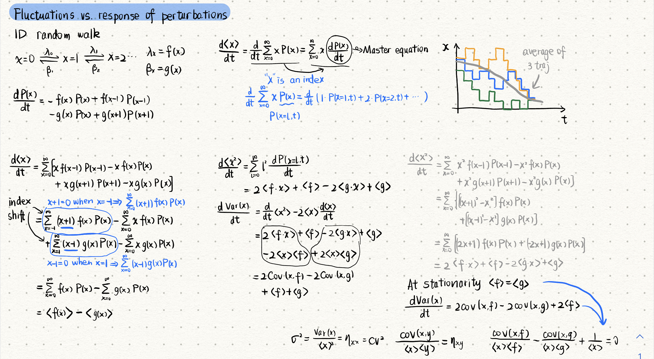
Always start from the simplest. Let’s consider a molecule $X$’s propensity (per unit time) of production and degradation by one molecule are $f(x)$ and $g(x)$. As a Markovian process, they merely depend on where the current state is. We write it as

where the probability on each grid is $P(x,t)$. The time evolution of the probability distribution $\frac{d}{dt}P(x,t)$ is described by a master equation, which can be interpreted as “plus the probability in and minus the probability out of that state”. It should be conditioned on the initial state, but we’ll drop it, because we’re interested in the stationary state, which all initial states will evolve to. From $\frac{d}{dt}P(x,t)$, using the “index shift” trick, we can get the evolution of statistical quantities of $X$.

Special case: constant birth and first-order degradation

Now, let’s look at an intuitive and simple case where the molecule has a constant production rate and a first-order degradation rate. The steady-state (also detailed balance in this case) of the probability distribution on grids forms a Poisson distribution.

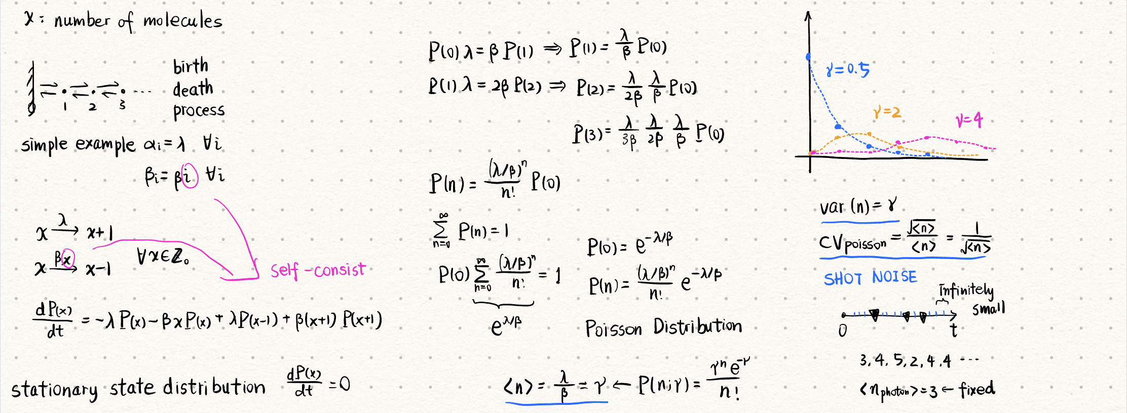
Note that for the stationary state, for each $x>0$ grid, the two ways in and two ways out should sum up to zero. While for the $x=0$ grid, there is only one way in and out from/to $x=1$ grid. Then we know ways $x=m$ to $x=m+1$ should equal $x=m+1$ to $x=m$, and it satisfies the detailed balance.

Of course, this is a linear reaction system and can be solved analytically by the generating function, see Solving the Poisson distribution with generating functions.

Multi-variable case

Gene regulatory networks consist of many interacting species. We consider a biochemical system with $n$ species and $m$ elementary reactions,

For this network, use the “index shift” trick to calculate mean, variances, and covariances with the master equation. The detailed steps are in [2], equation (1)-(3). I don’t bother to type the results here.

We follow the content in [2]. Define the vector of rate as $\mathbf{f}(\mathbf{x}):=\sum_i \mathbf{r}_i W_i(\mathbf{x})$.

Linear case

We can write the rate as $\mathbf{f}(\mathbf{x}(t)) = \mathbf{A}\mathbf{x}(t) + \mathbf{f}_0$, where $\mathbf{A}$ is an $n\times n$ real constant matrix (drift) and $\mathbf{f}_0$ is an $n$-dimensional constant vector.

Define the covariance matrix $\mathbf{\Sigma}(t):=\langle\mathbf{x}(t)\mathbf{x}^T(t)\rangle - \langle\mathbf{x}(t)\rangle \langle \mathbf{x}^T(t)\rangle$, autocorrelation $\mathbf{R}_{\mathbf{xx}}(t_1,t_2):=\langle\mathbf{x}(t_1)\mathbf{x}^T(t_2)\rangle - \langle\mathbf{x}(t_1)\rangle\langle\mathbf{x}^T(t_2)\rangle$. Following [5], there are some important exact results.

$\frac{d}{dt}\mathbf{\Sigma}(t) = \mathbf{A}\mathbf{\Sigma}(t) + \mathbf{\Sigma}\mathbf{A}(t)^T + \mathbf{D}(t)$. (5 in text, where $\mathbf{D}(t):=\sum_i\mathbf{r}_iW_i(\langle\mathbf{x}(t)\rangle)\mathbf{r}_i(t)$)

$\frac{\partial}{\partial t_1}\mathbf{R}{\mathbf{xx}}(t_1,t_2) = \mathbf{A}\mathbf{R}{\mathbf{xx}}(t_1,t_2)$. (7 in text)

For steady state,

• $\mathbf{A}\mathbf{R}{\mathbf{xx}}(0)+\mathbf{R}{\mathbf{xx}}(0)\mathbf{A}^T + \mathbf{D} = 0$ (9 in text). This is the Lyapunov equation (an exact result, not approximation), and often called the fluctuation-dissipation theorem, a balance between the tendency of particles to diffuse and mechanisms such as negative feedback that bring them back to equilibrium (Remark 3 in text).
• $\frac{\partial}{\partial\tau}\mathbf{R}{\mathbf{xx}}(\tau) = \mathbf{A}\mathbf{R}{\mathbf{xx}}(\tau)$ (10 in text). How to solve this system of ODEs? Use matrix exponential, which involves diagonalizing the matrix; see Linear Algebra (线性代数 - Matrix Exponential).

The classical model of mRNA and protein

This is an example of a linear case with the classical mRNA-protein model [1]. You can regard $X_1$ as the mRNA and $X_2$ as the protein. (In many cases, the protein degradation rate is very small compared with cell growth [6], and the dilution effects are often described as first-order degradation.) You will come across this model from time to time when you are reading Paulsson Group related things… For example, model [4] in [7], and equation [7] is the exact result of this linear rates model. See below how to derive.

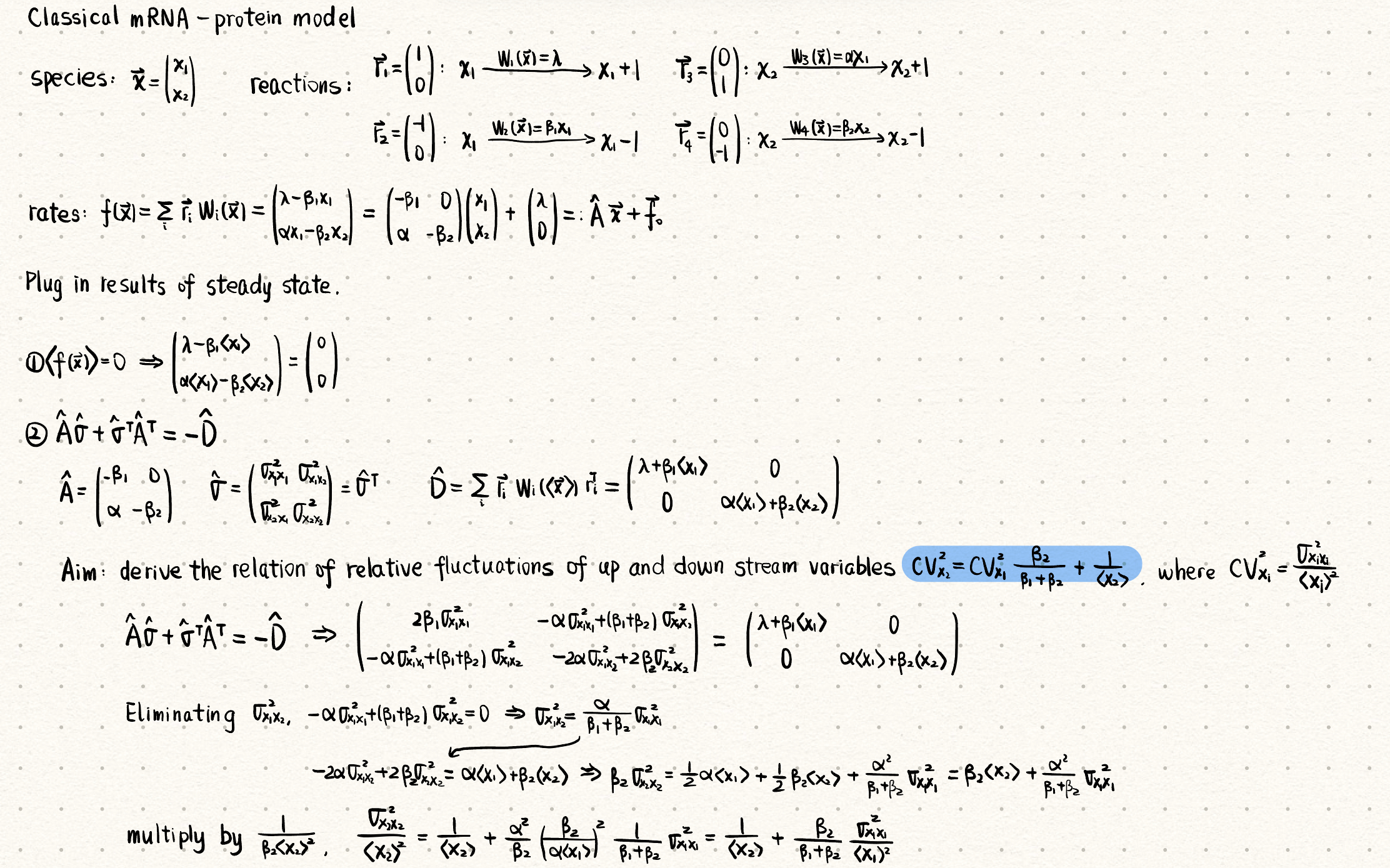
Again, this is a linear reaction system and can be solved analytically by the generating function, see [8]. In short, we write down the chemical master equation and use generating function to get the corresponding partial differential equation. Solving this PDE can be cumbersome, as shown in this paper!

The classical model with additional complex formation and disassociation

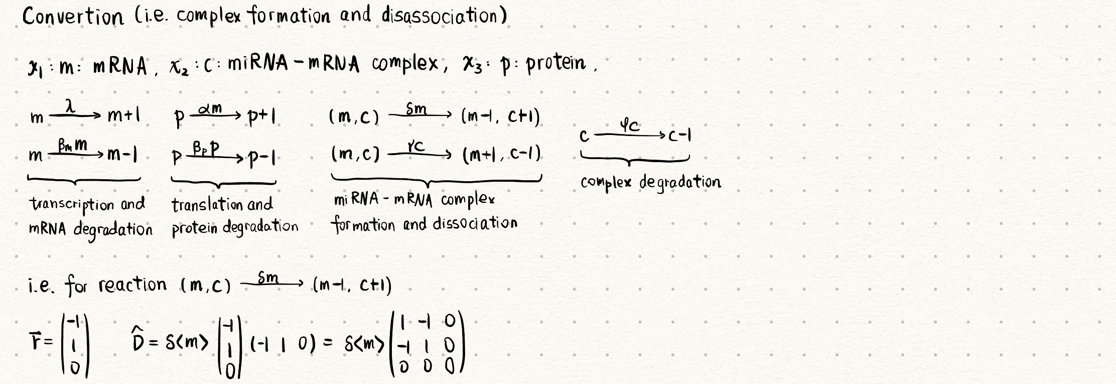
In [3], the role of the miRNA-mRNA complex in regulating noise at the protein level was considered. In Figure 1, I showed the matrix $\mathbf{D}$ of the reaction involving more than one species.

The “normalized” form

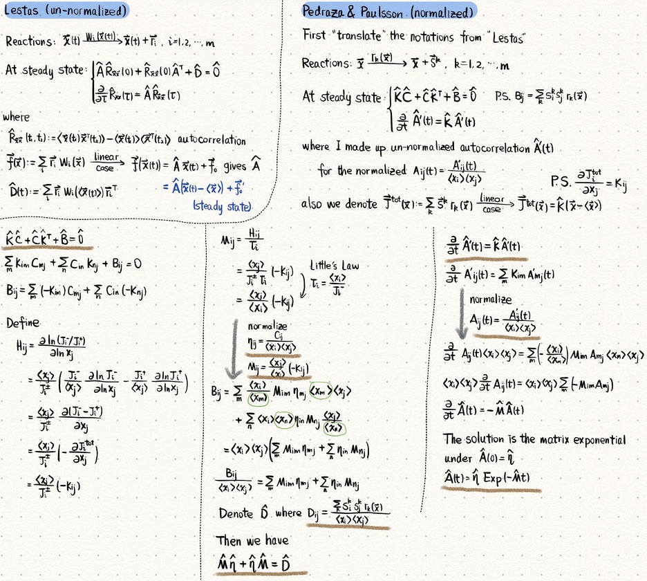
Well, I base the above derivation on [2]. In the well-known paper [3], where the author set up a “standard procedure”, they are in a normalized form (example papers using the “normalized” form: [3], [9], [10]). I show the procedure to normalize them in Figure 2. Note that “Little’s Law” is applied here.

Wrap up

I sincerely thank everyone in my group, especially B Kell and A. Hilfinger. You can regard this post as my first-year progress in theory, although it should not have taken that long…. I feel like I’m just crossing the critical point. I completed a phase transition of “being defeated by the equations from the beginning of papers” to “understand the basic math and have a better sense of deriving statistical properties.”

References

1. M. Thattai and A. van Oudenaarden. Intrinsic noise in gene regulatory networks. Proceedings of the National Academy of Sciences, 98(15), 8614–8619, 2001. DOI
2. I. Lestas, J. Paulsson, N. E. Ross, and G. Vinnicombe. Noise in Gene Regulatory Networks. IEEE Transactions on Automatic Control, 53(Special Issue), 189–200, 2008. DOI
3. J. Paulsson. Summing up the noise in gene networks. Nature, 427(6973), 415–418, 2004. DOI
4. M. B. Elowitz, A. J. Levine, E. D. Siggia, and P. S. Swain. Stochastic Gene Expression in a Single Cell. Science, 297(5584), 1183–1186, 2002. DOI
5. J. Paulsson. Models of stochastic gene expression. Physics of Life Reviews, 2(2), 157–175, 2005. DOI
6. A. L. Koch and H. R. Levy. Protein turnover in growing cultures of Escherichia coli. The Journal of Biological Chemistry, 217(2), 947–957, 1955.
7. A. Hilfinger and J. Paulsson. Separating intrinsic from extrinsic fluctuations in dynamic biological systems. Proceedings of the National Academy of Sciences, 108(29), 12167–12172, 2011. DOI
8. P. Bokes and others. Exact and approximate distributions of protein and mRNA levels in the low-copy regime of gene expression. Journal of Mathematical Biology, 64(5), 829–854, 2012. DOI
9. R. Fan and A. Hilfinger. The effect of microRNA on protein variability and gene expression fidelity. Biophysical Journal, 122(5), 905–923, 2023. Online
10. J. M. Pedraza and J. Paulsson. Effects of molecular memory and bursting on fluctuations in gene expression. Science, 319(5861), 339–343, 2008.
11. N. G. van Kampen. Stochastic Processes in Physics and Chemistry. 1, Elsevier, 1992.
12. Lyapunov equation. Wikipedia, 2023. Online