Given a system of nonlinear ODEs that generates a limit cycle oscillation, can we find out the period and the extrema of the variables, without numerically solving the ODEs in time?

Van der Pol oscillator

Python code computation example: vanderpol.ipynb.

Van der Pol oscillator’s ODEs: $\frac{d^2x}{dt^2}-\mu(1-x^2)\frac{dx}{dt}+x=0$. To convert to first-order derivatives, set $y=\frac{dx}{dt}$, then the ODEs become

The analysis follows (En) Nonlinear Dynamics. Denote $ \vec u=[x,y]^T$, and the ODEs $\frac{d\vec u}{dt}=\vec f(\vec u)$.

It has one fixed point $\vec u_0=[0,0]^T$. The Jacobian matrix is

At the fixed point $\vec u_0$, the Jacobian is

To analyze the stability, calculate the eigenvalue by $\det\lambda\hat I-\hat J(\vec u_0)=0$, which gives $\lambda=\frac{\mu\pm\sqrt{\mu^2-4}}{2}$.

For parameter $\mu>0$, we can see the eigenvalue always has a positive real part, which means the fixed point is unstable. For $0<\mu<2$, $\lambda=\frac{\mu\pm i\sqrt{4-\mu^2}}{2}$, and the fixed point is an unstable spiral; for $\mu>2$, the fixed point is an unstable node. In both case, the ODEs behave as a limit cycle oscillator. (Actually I’m a bit shocked that the unstable node case still behaves as limit cycle oscillation… I need to revisit nonlinear dynamics…)

In the following part, I will take the parameter as $\mu=1$.

Numerical simulation

We simulate the system from the initial condition $\vec u(0)=[0,1]^T$,

solve the ODEs by RK4 (in my example, I showed both handwritten RK4 and using scipy module). Below are the $(x,y)-t$ plot and $(x,y)$ plot.

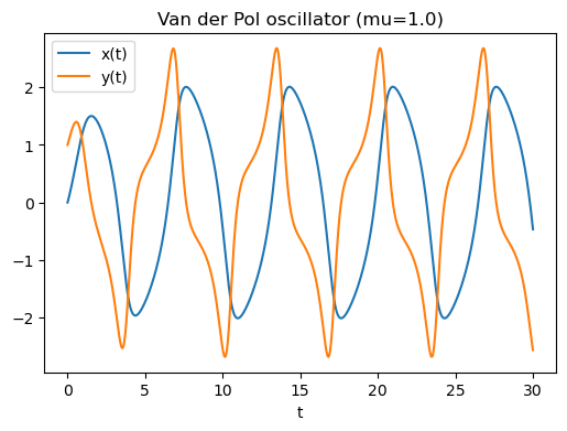
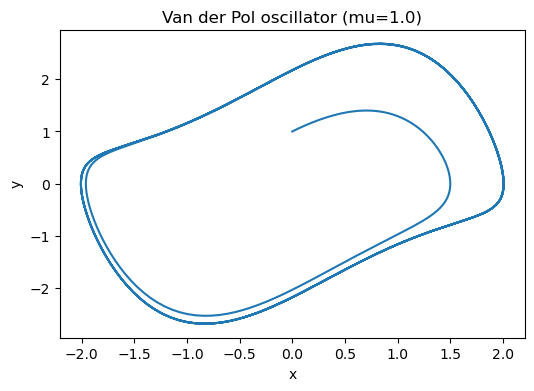
We can see the limit cycle oscillation, with period $T$ around 5~10, and maximum & minimum $x$ around $\pm$ 2, maximum & minimum $y$ around $\pm$ 2.8.

Here comes a question: If I want to find the period and the extrema of variables without numerically solving ODEs and “eyeballing” (or write a code to “eyeball”) the solutions?

Find $T$

It comes to solve a boundary value problem (BVP)

To determine this solution, we need to fix the starting point called $\vec u(0)$ on the closed oscillating trajectory. Then solving the above BVP boils down to solve

where $[x(T)-x(0),y(T)-y(0)]^T=\int_0^{T}\vec f(\vec u(t))dt-\vec u(0)$, and $y(0)$ chosen here to determine $\vec u(0)$. The problem is to find the root of $\vec g([x(0),y(0),T])^T$ since $y(0)=0$ is indeed on the trajectory.

To solve this, we use multi-variable version Newton-Raphson method. If we have $[x_k(0),y_k(0),T_k]^T$,

we can use

to solve $\vec\Delta$, then update

In the Jupyter notebook, we show that the solution is

x0=2.00861986, y0=0.00000000,  T=6.66328686.

However, this method doesn’t guarantee that the residue will converge to zero with random initial guess. Also, even if the residues successfully converge to zero, the period $T$ and converge to $nT$ ($n\in \mathbb Z^+$) with the initial guess near that $nT$. Examples are in the corresponding Jupyter notebook.

Usually, you expect it to work well when your initial guess is close enough to the true solution. But what is the point if I already know the solution and throw in the initial “guess” based on that? This can be useful for parameter scanning. Given a system, you continuously vary one parameter within a range, to find the value that give you the desired properties, e.g., $T$ or extrema. According to the implicit function theorem (IFT) (please refer to Lecture Notes on Numerical Analysis of Nonlinear Equations), these properties also vary continuously with the parameter. So, you can get the “correct” guess for initial values for one parameter, and you vary the parameter a little bit, and throw in the previous guess (close to the correct result) to get the new solution…

Find extrema of

What about the extrema on the trajectory of all variables? (Here we regard $x$ and $y$ in the van der Pol oscillator as two variables to show the computation routine).

From above, we’ve found one point on the trajectory and the period $T$, then we can sample one period and find the extrema. The idea is easy, simulate one period to find the extrema by tracking the values of each variable.

In the Jupyter notebook, we show that the solution is

var 0: max=2.006393 at t=3.331643, min=-2.008620 at t=3.331644
var 1: max=2.678441 at t=5.839207, min=-2.678441 at t=2.507564.